Data Loading and Processing Tutorial

Author: Sasank Chilamkurthy

A lot of effort in solving any machine learning problem goes in to preparing the data. PyTorch provides many tools to make data loading easy and hopefully, to make your code more readable. In this tutorial, we will see how to load and preprocess/augment data from a non trivial dataset.

To run this tutorial, please make sure the following packages are installed:

• scikit-image: For image io and transforms
• pandas: For easier csv parsing

from __future__ import print_function, division
import os
import torch
import pandas as pd
from skimage import io, transform
import numpy as np
import matplotlib.pyplot as plt
from torch.utils.data import Dataset, DataLoader
from torchvision import transforms, utils

# Ignore warnings
import warnings
warnings.filterwarnings("ignore")

plt.ion()   # interactive mode

The dataset we are going to deal with is that of facial pose. This means that a face is annotated like this:

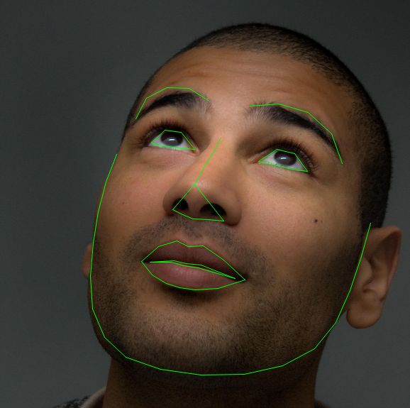
Over all, 68 different landmark points are annotated for each face.

Note

Download the dataset from here so that the images are in a directory named ‘faces/’. This dataset was actually generated by applying excellent dlib’s pose estimation on a few images from imagenet tagged as ‘face’.

Dataset comes with a csv file with annotations which looks like this:

image_name,part_0_x,part_0_y,part_1_x,part_1_y,part_2_x, ... ,part_67_x,part_67_y
0805personali01.jpg,27,83,27,98, ... 84,134
1084239450_e76e00b7e7.jpg,70,236,71,257, ... ,128,312

Let’s quickly read the CSV and get the annotations in an (N, 2) array where N is the number of landmarks.

landmarks_frame = pd.read_csv('faces/face_landmarks.csv')

n = 65
img_name = landmarks_frame.iloc[n, 0]
landmarks = landmarks_frame.iloc[n, 1:].as_matrix()
landmarks = landmarks.astype('float').reshape(-1, 2)

print('Image name: {}'.format(img_name))
print('Landmarks shape: {}'.format(landmarks.shape))
print('First 4 Landmarks: {}'.format(landmarks[:4]))

Out:

Image name: person-7.jpg
Landmarks shape: (68, 2)
First 4 Landmarks: [[32. 65.]
 [33. 76.]
 [34. 86.]
 [34. 97.]]

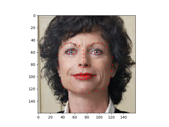
Let’s write a simple helper function to show an image and its landmarks and use it to show a sample.

def show_landmarks(image, landmarks):
    """Show image with landmarks"""
    plt.imshow(image)
    plt.scatter(landmarks[:, 0], landmarks[:, 1], s=10, marker='.', c='r')
    plt.pause(0.001)  # pause a bit so that plots are updated

plt.figure()
show_landmarks(io.imread(os.path.join('faces/', img_name)),
               landmarks)
plt.show()

Dataset class

torch.utils.data.Dataset is an abstract class representing a dataset. Your custom dataset should inherit Dataset and override the following methods:

• __len__ so that len(dataset) returns the size of the dataset.
• __getitem__ to support the indexing such that dataset[i] can be used to get \(i\)th sample

Let’s create a dataset class for our face landmarks dataset. We will read the csv in __init__ but leave the reading of images to __getitem__. This is memory efficient because all the images are not stored in the memory at once but read as required.

Sample of our dataset will be a dict {'image': image, 'landmarks': landmarks}. Our datset will take an optional argument transform so that any required processing can be applied on the sample. We will see the usefulness of transform in the next section.

class FaceLandmarksDataset(Dataset):
    """Face Landmarks dataset."""

    def __init__(self, csv_file, root_dir, transform=None):
        """
        Args:
            csv_file (string): Path to the csv file with annotations.
            root_dir (string): Directory with all the images.
            transform (callable, optional): Optional transform to be applied
                on a sample.
        """
        self.landmarks_frame = pd.read_csv(csv_file)
        self.root_dir = root_dir
        self.transform = transform

    def __len__(self):
        return len(self.landmarks_frame)

    def __getitem__(self, idx):
        img_name = os.path.join(self.root_dir,
                                self.landmarks_frame.iloc[idx, 0])
        image = io.imread(img_name)
        landmarks = self.landmarks_frame.iloc[idx, 1:].as_matrix()
        landmarks = landmarks.astype('float').reshape(-1, 2)
        sample = {'image': image, 'landmarks': landmarks}

        if self.transform:
            sample = self.transform(sample)

        return sample

Let’s instantiate this class and iterate through the data samples. We will print the sizes of first 4 samples and show their landmarks.

face_dataset = FaceLandmarksDataset(csv_file='faces/face_landmarks.csv',
                                    root_dir='faces/')

fig = plt.figure()

for i in range(len(face_dataset)):
    sample = face_dataset[i]

    print(i, sample['image'].shape, sample['landmarks'].shape)

    ax = plt.subplot(1, 4, i + 1)
    plt.tight_layout()
    ax.set_title('Sample #{}'.format(i))
    ax.axis('off')
    show_landmarks(**sample)

    if i == 3:
        plt.show()
        break

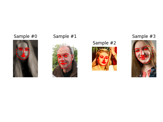
Out:

0 (324, 215, 3) (68, 2)
1 (500, 333, 3) (68, 2)
2 (250, 258, 3) (68, 2)
3 (434, 290, 3) (68, 2)

Transforms

One issue we can see from the above is that the samples are not of the same size. Most neural networks expect the images of a fixed size. Therefore, we will need to write some prepocessing code. Let’s create three transforms:

• Rescale: to scale the image
• RandomCrop: to crop from image randomly. This is data augmentation.
• ToTensor: to convert the numpy images to torch images (we need to swap axes).

We will write them as callable classes instead of simple functions so that parameters of the transform need not be passed everytime it’s called. For this, we just need to implement __call__ method and if required, __init__ method. We can then use a transform like this:

tsfm = Transform(params)
transformed_sample = tsfm(sample)

Observe below how these transforms had to be applied both on the image and landmarks.

class Rescale(object):
    """Rescale the image in a sample to a given size.

    Args:
        output_size (tuple or int): Desired output size. If tuple, output is
            matched to output_size. If int, smaller of image edges is matched
            to output_size keeping aspect ratio the same.
    """

    def __init__(self, output_size):
        assert isinstance(output_size, (int, tuple))
        self.output_size = output_size

    def __call__(self, sample):
        image, landmarks = sample['image'], sample['landmarks']

        h, w = image.shape[:2]
        if isinstance(self.output_size, int):
            if h > w:
                new_h, new_w = self.output_size * h / w, self.output_size
            else:
                new_h, new_w = self.output_size, self.output_size * w / h
        else:
            new_h, new_w = self.output_size

        new_h, new_w = int(new_h), int(new_w)

        img = transform.resize(image, (new_h, new_w))

        # h and w are swapped for landmarks because for images,
        # x and y axes are axis 1 and 0 respectively
        landmarks = landmarks * [new_w / w, new_h / h]

        return {'image': img, 'landmarks': landmarks}


class RandomCrop(object):
    """Crop randomly the image in a sample.

    Args:
        output_size (tuple or int): Desired output size. If int, square crop
            is made.
    """

    def __init__(self, output_size):
        assert isinstance(output_size, (int, tuple))
        if isinstance(output_size, int):
            self.output_size = (output_size, output_size)
        else:
            assert len(output_size) == 2
            self.output_size = output_size

    def __call__(self, sample):
        image, landmarks = sample['image'], sample['landmarks']

        h, w = image.shape[:2]
        new_h, new_w = self.output_size

        top = np.random.randint(0, h - new_h)
        left = np.random.randint(0, w - new_w)

        image = image[top: top + new_h,
                      left: left + new_w]

        landmarks = landmarks - [left, top]

        return {'image': image, 'landmarks': landmarks}


class ToTensor(object):
    """Convert ndarrays in sample to Tensors."""

    def __call__(self, sample):
        image, landmarks = sample['image'], sample['landmarks']

        # swap color axis because
        # numpy image: H x W x C
        # torch image: C X H X W
        image = image.transpose((2, 0, 1))
        return {'image': torch.from_numpy(image),
                'landmarks': torch.from_numpy(landmarks)}

Compose transforms

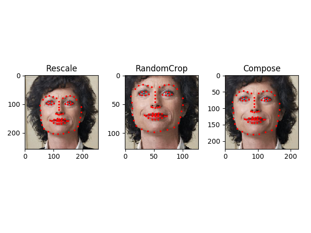
Now, we apply the transforms on an sample.

Let’s say we want to rescale the shorter side of the image to 256 and then randomly crop a square of size 224 from it. i.e, we want to compose Rescale and RandomCrop transforms. torchvision.transforms.Compose is a simple callable class which allows us to do this.

scale = Rescale(256)
crop = RandomCrop(128)
composed = transforms.Compose([Rescale(256),
                               RandomCrop(224)])

# Apply each of the above transforms on sample.
fig = plt.figure()
sample = face_dataset[65]
for i, tsfrm in enumerate([scale, crop, composed]):
    transformed_sample = tsfrm(sample)

    ax = plt.subplot(1, 3, i + 1)
    plt.tight_layout()
    ax.set_title(type(tsfrm).__name__)
    show_landmarks(**transformed_sample)

plt.show()

Iterating through the dataset

Let’s put this all together to create a dataset with composed transforms. To summarize, every time this dataset is sampled:

• An image is read from the file on the fly
• Transforms are applied on the read image
• Since one of the transforms is random, data is augmentated on sampling

We can iterate over the created dataset with a for i in range loop as before.

transformed_dataset = FaceLandmarksDataset(csv_file='faces/face_landmarks.csv',
                                           root_dir='faces/',
                                           transform=transforms.Compose([
                                               Rescale(256),
                                               RandomCrop(224),
                                               ToTensor()
                                           ]))

for i in range(len(transformed_dataset)):
    sample = transformed_dataset[i]

    print(i, sample['image'].size(), sample['landmarks'].size())

    if i == 3:
        break

Out:

0 torch.Size([3, 224, 224]) torch.Size([68, 2])
1 torch.Size([3, 224, 224]) torch.Size([68, 2])
2 torch.Size([3, 224, 224]) torch.Size([68, 2])
3 torch.Size([3, 224, 224]) torch.Size([68, 2])

However, we are losing a lot of features by using a simple for loop to iterate over the data. In particular, we are missing out on:

• Batching the data
• Shuffling the data
• Load the data in parallel using multiprocessing workers.

torch.utils.data.DataLoader is an iterator which provides all these features. Parameters used below should be clear. One parameter of interest is collate_fn. You can specify how exactly the samples need to be batched using collate_fn. However, default collate should work fine for most use cases.

dataloader = DataLoader(transformed_dataset, batch_size=4,
                        shuffle=True, num_workers=4)


# Helper function to show a batch
def show_landmarks_batch(sample_batched):
    """Show image with landmarks for a batch of samples."""
    images_batch, landmarks_batch = \
            sample_batched['image'], sample_batched['landmarks']
    batch_size = len(images_batch)
    im_size = images_batch.size(2)

    grid = utils.make_grid(images_batch)
    plt.imshow(grid.numpy().transpose((1, 2, 0)))

    for i in range(batch_size):
        plt.scatter(landmarks_batch[i, :, 0].numpy() + i * im_size,
                    landmarks_batch[i, :, 1].numpy(),
                    s=10, marker='.', c='r')

        plt.title('Batch from dataloader')

for i_batch, sample_batched in enumerate(dataloader):
    print(i_batch, sample_batched['image'].size(),
          sample_batched['landmarks'].size())

    # observe 4th batch and stop.
    if i_batch == 3:
        plt.figure()
        show_landmarks_batch(sample_batched)
        plt.axis('off')
        plt.ioff()
        plt.show()
        break

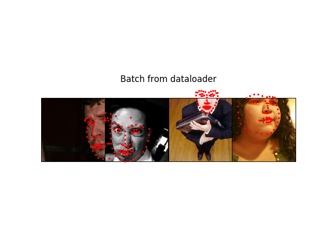
Out:

0 torch.Size([4, 3, 224, 224]) torch.Size([4, 68, 2])
1 torch.Size([4, 3, 224, 224]) torch.Size([4, 68, 2])
2 torch.Size([4, 3, 224, 224]) torch.Size([4, 68, 2])
3 torch.Size([4, 3, 224, 224]) torch.Size([4, 68, 2])

Afterword: torchvision

In this tutorial, we have seen how to write and use datasets, transforms and dataloader. torchvision package provides some common datasets and transforms. You might not even have to write custom classes. One of the more generic datasets available in torchvision is ImageFolder. It assumes that images are organized in the following way:

root/ants/xxx.png
root/ants/xxy.jpeg
root/ants/xxz.png
.
.
.
root/bees/123.jpg
root/bees/nsdf3.png
root/bees/asd932_.png

where ‘ants’, ‘bees’ etc. are class labels. Similarly generic transforms which operate on PIL.Image like RandomHorizontalFlip, Scale, are also avaiable. You can use these to write a dataloader like this:

import torch
from torchvision import transforms, datasets

data_transform = transforms.Compose([
        transforms.RandomSizedCrop(224),
        transforms.RandomHorizontalFlip(),
        transforms.ToTensor(),
        transforms.Normalize(mean=[0.485, 0.456, 0.406],
                             std=[0.229, 0.224, 0.225])
    ])
hymenoptera_dataset = datasets.ImageFolder(root='hymenoptera_data/train',
                                           transform=data_transform)
dataset_loader = torch.utils.data.DataLoader(hymenoptera_dataset,
                                             batch_size=4, shuffle=True,
                                             num_workers=4)

For an example with training code, please see 전이학습(Transfer Learning) 튜토리얼.

Total running time of the script: ( 0 minutes 58.933 seconds)