Spatial Transformer Networks Tutorial
Author: Ghassen HAMROUNI
In this tutorial, you will learn how to augment your network using a visual attention mechanism called spatial transformer networks. You can read more about the spatial transformer networks in the DeepMind paper
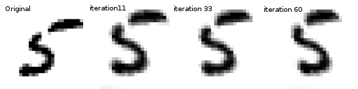
Spatial transformer networks are a generalization of differentiable attention to any spatial transformation. Spatial transformer networks (STN for short) allow a neural network to learn how to perform spatial transformations on the input image in order to enhance the geometric invariance of the model. For example, it can crop a region of interest, scale and correct the orientation of an image. It can be a useful mechanism because CNNs are not invariant to rotation and scale and more general affine transformations.
One of the best things about STN is the ability to simply plug it into any existing CNN with very little modification.
# License: BSD
# Author: Ghassen Hamrouni

from __future__ import print_function
import torch
import torch.nn as nn
import torch.nn.functional as F
import torch.optim as optim
import torchvision
from torchvision import datasets, transforms
from torch.autograd import Variable
import matplotlib.pyplot as plt
import numpy as np

plt.ion()   # interactive mode
Loading the data
In this post we experiment with the classic MNIST dataset. Using a standard convolutional network augmented with a spatial transformer network.
use_cuda = torch.cuda.is_available()

# Training dataset
train_loader = torch.utils.data.DataLoader(
    datasets.MNIST(root='.', train=True, download=True,
                   transform=transforms.Compose([
                       transforms.ToTensor(),
                       transforms.Normalize((0.1307,), (0.3081,))
                   ])), batch_size=64, shuffle=True, num_workers=4)
# Test dataset
test_loader = torch.utils.data.DataLoader(
    datasets.MNIST(root='.', train=False, transform=transforms.Compose([
        transforms.ToTensor(),
        transforms.Normalize((0.1307,), (0.3081,))
    ])), batch_size=64, shuffle=True, num_workers=4)
Out:
Downloading http://yann.lecun.com/exdb/mnist/train-images-idx3-ubyte.gz
Downloading http://yann.lecun.com/exdb/mnist/train-labels-idx1-ubyte.gz
Downloading http://yann.lecun.com/exdb/mnist/t10k-images-idx3-ubyte.gz
Downloading http://yann.lecun.com/exdb/mnist/t10k-labels-idx1-ubyte.gz
Processing...
Done!
Depicting spatial transformer networks
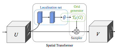
Spatial transformer networks boils down to three main components :
- The localization network is a regular CNN which regresses the transformation parameters. The transformation is never learned explicitly from this dataset, instead the network learns automatically the spatial transformations that enhances the global accuracy.
- The grid generator generates a grid of coordinates in the input image corresponding to each pixel from the output image.
- The sampler uses the parameters of the transformation and applies it to the input image.
Note
We need the latest version of PyTorch that contains affine_grid and grid_sample modules.
class Net(nn.Module):
    def __init__(self):
        super(Net, self).__init__()
        self.conv1 = nn.Conv2d(1, 10, kernel_size=5)
        self.conv2 = nn.Conv2d(10, 20, kernel_size=5)
        self.conv2_drop = nn.Dropout2d()
        self.fc1 = nn.Linear(320, 50)
        self.fc2 = nn.Linear(50, 10)

        # Spatial transformer localization-network
        self.localization = nn.Sequential(
            nn.Conv2d(1, 8, kernel_size=7),
            nn.MaxPool2d(2, stride=2),
            nn.ReLU(True),
            nn.Conv2d(8, 10, kernel_size=5),
            nn.MaxPool2d(2, stride=2),
            nn.ReLU(True)
        )

        # Regressor for the 3 * 2 affine matrix
        self.fc_loc = nn.Sequential(
            nn.Linear(10 * 3 * 3, 32),
            nn.ReLU(True),
            nn.Linear(32, 3 * 2)
        )

        # Initialize the weights/bias with identity transformation
        self.fc_loc[2].weight.data.fill_(0)
        self.fc_loc[2].bias.data = torch.FloatTensor([1, 0, 0, 0, 1, 0])

    # Spatial transformer network forward function
    def stn(self, x):
        xs = self.localization(x)
        xs = xs.view(-1, 10 * 3 * 3)
        theta = self.fc_loc(xs)
        theta = theta.view(-1, 2, 3)

        grid = F.affine_grid(theta, x.size())
        x = F.grid_sample(x, grid)

        return x

    def forward(self, x):
        # transform the input
        x = self.stn(x)

        # Perform the usual forward pass
        x = F.relu(F.max_pool2d(self.conv1(x), 2))
        x = F.relu(F.max_pool2d(self.conv2_drop(self.conv2(x)), 2))
        x = x.view(-1, 320)
        x = F.relu(self.fc1(x))
        x = F.dropout(x, training=self.training)
        x = self.fc2(x)
        return F.log_softmax(x, dim=1)


model = Net()
if use_cuda:
    model.cuda()
Training the model
Now, let’s use the SGD algorithm to train the model. The network is learning the classification task in a supervised way. In the same time the model is learning STN automatically in an end-to-end fashion.
optimizer = optim.SGD(model.parameters(), lr=0.01)


def train(epoch):
    model.train()
    for batch_idx, (data, target) in enumerate(train_loader):
        if use_cuda:
            data, target = data.cuda(), target.cuda()

        data, target = Variable(data), Variable(target)
        optimizer.zero_grad()
        output = model(data)
        loss = F.nll_loss(output, target)
        loss.backward()
        optimizer.step()
        if batch_idx % 500 == 0:
            print('Train Epoch: {} [{}/{} ({:.0f}%)]\tLoss: {:.6f}'.format(
                epoch, batch_idx * len(data), len(train_loader.dataset),
                100. * batch_idx / len(train_loader), loss.data[0]))
#
# A simple test procedure to measure STN the performances on MNIST.
#


def test():
    model.eval()
    test_loss = 0
    correct = 0
    for data, target in test_loader:
        if use_cuda:
            data, target = data.cuda(), target.cuda()
        data, target = Variable(data, volatile=True), Variable(target)
        output = model(data)

        # sum up batch loss
        test_loss += F.nll_loss(output, target, size_average=False).data[0]
        # get the index of the max log-probability
        pred = output.data.max(1, keepdim=True)[1]
        correct += pred.eq(target.data.view_as(pred)).cpu().sum()

    test_loss /= len(test_loader.dataset)
    print('\nTest set: Average loss: {:.4f}, Accuracy: {}/{} ({:.0f}%)\n'
          .format(test_loss, correct, len(test_loader.dataset),
                  100. * correct / len(test_loader.dataset)))
Visualizing the STN results
Now, we will inspect the results of our learned visual attention mechanism.
We define a small helper function in order to visualize the transformations while training.
def convert_image_np(inp):
"""Convert a Tensor to numpy image."""
inp = inp.numpy().transpose((1, 2, 0))
mean = np.array([0.485, 0.456, 0.406])
std = np.array([0.229, 0.224, 0.225])
inp = std * inp + mean
inp = np.clip(inp, 0, 1)
return inp
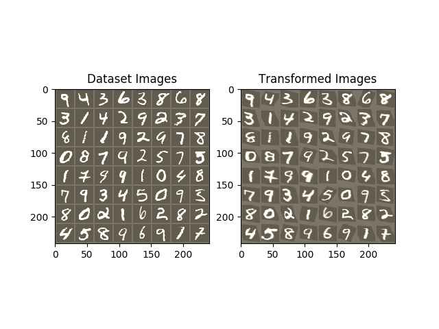
# We want to visualize the output of the spatial transformers layer
# after the training, we visualize a batch of input images and
# the corresponding transformed batch using STN.
def visualize_stn():
# Get a batch of training data
data, _ = next(iter(test_loader))
data = Variable(data, volatile=True)
if use_cuda:
data = data.cuda()
input_tensor = data.cpu().data
transformed_input_tensor = model.stn(data).cpu().data
in_grid = convert_image_np(
torchvision.utils.make_grid(input_tensor))
out_grid = convert_image_np(
torchvision.utils.make_grid(transformed_input_tensor))
# Plot the results side-by-side
f, axarr = plt.subplots(1, 2)
axarr[0].imshow(in_grid)
axarr[0].set_title('Dataset Images')
axarr[1].imshow(out_grid)
axarr[1].set_title('Transformed Images')
for epoch in range(1, 20 + 1):
train(epoch)
test()
# Visualize the STN transformation on some input batch
visualize_stn()
plt.ioff()
plt.show()
Out:
Train Epoch: 1 [0/60000 (0%)]   Loss: 2.342094
Train Epoch: 1 [32000/60000 (53%)]      Loss: 0.914849

Test set: Average loss: 0.1988, Accuracy: 9407/10000 (94%)

Train Epoch: 2 [0/60000 (0%)]   Loss: 0.727430
Train Epoch: 2 [32000/60000 (53%)]      Loss: 0.518599

Test set: Average loss: 0.1311, Accuracy: 9586/10000 (96%)

Train Epoch: 3 [0/60000 (0%)]   Loss: 0.286077
Train Epoch: 3 [32000/60000 (53%)]      Loss: 0.178694

Test set: Average loss: 0.0941, Accuracy: 9711/10000 (97%)

Train Epoch: 4 [0/60000 (0%)]   Loss: 0.163664
Train Epoch: 4 [32000/60000 (53%)]      Loss: 0.260930

Test set: Average loss: 0.0781, Accuracy: 9767/10000 (98%)

Train Epoch: 5 [0/60000 (0%)]   Loss: 0.201850
Train Epoch: 5 [32000/60000 (53%)]      Loss: 0.231272

Test set: Average loss: 0.0716, Accuracy: 9789/10000 (98%)

Train Epoch: 6 [0/60000 (0%)]   Loss: 0.104988
Train Epoch: 6 [32000/60000 (53%)]      Loss: 0.104964

Test set: Average loss: 0.0595, Accuracy: 9809/10000 (98%)

Train Epoch: 7 [0/60000 (0%)]   Loss: 0.047372
Train Epoch: 7 [32000/60000 (53%)]      Loss: 0.083524

Test set: Average loss: 0.0587, Accuracy: 9824/10000 (98%)

Train Epoch: 8 [0/60000 (0%)]   Loss: 0.110441
Train Epoch: 8 [32000/60000 (53%)]      Loss: 0.057427

Test set: Average loss: 0.0724, Accuracy: 9799/10000 (98%)

Train Epoch: 9 [0/60000 (0%)]   Loss: 0.121870
Train Epoch: 9 [32000/60000 (53%)]      Loss: 0.165922

Test set: Average loss: 0.0577, Accuracy: 9815/10000 (98%)

Train Epoch: 10 [0/60000 (0%)]  Loss: 0.054281
Train Epoch: 10 [32000/60000 (53%)]     Loss: 0.183995

Test set: Average loss: 0.0615, Accuracy: 9804/10000 (98%)

Train Epoch: 11 [0/60000 (0%)]  Loss: 0.112812
Train Epoch: 11 [32000/60000 (53%)]     Loss: 0.041237

Test set: Average loss: 0.0619, Accuracy: 9803/10000 (98%)

Train Epoch: 12 [0/60000 (0%)]  Loss: 0.091255
Train Epoch: 12 [32000/60000 (53%)]     Loss: 0.054673

Test set: Average loss: 0.0434, Accuracy: 9862/10000 (99%)

Train Epoch: 13 [0/60000 (0%)]  Loss: 0.087725
Train Epoch: 13 [32000/60000 (53%)]     Loss: 0.136220

Test set: Average loss: 0.0440, Accuracy: 9853/10000 (99%)

Train Epoch: 14 [0/60000 (0%)]  Loss: 0.023782
Train Epoch: 14 [32000/60000 (53%)]     Loss: 0.043973

Test set: Average loss: 0.0463, Accuracy: 9857/10000 (99%)

Train Epoch: 15 [0/60000 (0%)]  Loss: 0.187337
Train Epoch: 15 [32000/60000 (53%)]     Loss: 0.204377

Test set: Average loss: 0.0496, Accuracy: 9850/10000 (98%)

Train Epoch: 16 [0/60000 (0%)]  Loss: 0.045294
Train Epoch: 16 [32000/60000 (53%)]     Loss: 0.027516

Test set: Average loss: 0.0444, Accuracy: 9871/10000 (99%)

Train Epoch: 17 [0/60000 (0%)]  Loss: 0.039108
Train Epoch: 17 [32000/60000 (53%)]     Loss: 0.119702

Test set: Average loss: 0.0486, Accuracy: 9845/10000 (98%)

Train Epoch: 18 [0/60000 (0%)]  Loss: 0.200034
Train Epoch: 18 [32000/60000 (53%)]     Loss: 0.140622

Test set: Average loss: 0.0425, Accuracy: 9871/10000 (99%)

Train Epoch: 19 [0/60000 (0%)]  Loss: 0.091878
Train Epoch: 19 [32000/60000 (53%)]     Loss: 0.087307

Test set: Average loss: 0.0369, Accuracy: 9886/10000 (99%)

Train Epoch: 20 [0/60000 (0%)]  Loss: 0.078879
Train Epoch: 20 [32000/60000 (53%)]     Loss: 0.104612

Test set: Average loss: 0.0454, Accuracy: 9863/10000 (99%)
Total running time of the script: ( 1 minutes 33.840 seconds)