nn 패키지

nn 패키지는 autograd를 완벽하게 통합하기 위해 재설계(redesign)하였습니다. 무엇이 변경되었는지 살펴보겠습니다.

autograd로 컨테이너(container)를 교체:

ConcatTable 같은 컨테이너나 CAddTable 같은 모듈, 또는 nngraph를 사용하거나 디버깅하기 위한 컨테이너들은 이제 더 이상 사용하지 않습니다. 대신 더 깔끔한 autograd를 사용해서 신경망을 정의할 것입니다. 예를 들면,

• output = nn.CAddTable():forward({input1, input2}) 대신, output = input1 + input2 를 사용합니다.
• output = nn.MulConstant(0.5):forward(input) 대신, output = input * 0.5 를 사용합니다.

상태(state)는 모듈 내에 저장되지 않고, 신경망 그래프 상에 존재합니다:

덕분에 순환신경망을 사용하는 방법이 더 간단해졌습니다. 이제 순환신경망을 만들 때, 더 이상 가중치(weight) 공유에 대해서는 생각할 필요 없이 동일한 Linear 계층(layer)을 여러 차례 호출하면 됩니다.

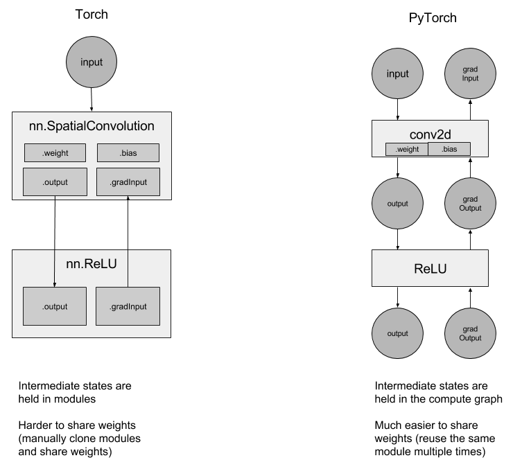
torch-nn-vs-pytorch-nn

간소화된 디버깅(debugging):

디버깅은 Python의 pdb 디버거를 사용하여 직관적이며, 디버거와 스택 추적(stack trace)은 에러가 발생한 곳에서 정확히 멈춥니다. 이제 보이는대로 얻을 것입니다. (What you see is what you get.)

예제1: 합성곱 신경망(ConvNet)

이제 어떻게 작은 합성곱 신경망을 만드는지 살펴보겠습니다.

모든 신경망은 기본(base) 클래스인 nn.Module 로부터 파생됩니다:

• 생성자(constructor)에서, 사용할 모든 계층(layer)을 선언합니다.
• 순전파(forward) 함수에서, 신경망 모델이 입력에서 출력까지 어떻게 실행되는지를 정의합니다.

import torch
import torch.nn as nn
import torch.nn.functional as F


class MNISTConvNet(nn.Module):

    def __init__(self):
        # 여기에서모든 모듈을 초기화해놓고,
        # 나중에 여기에 선언한 이름으로 접근할 수 있습니다.
        super(MNISTConvNet, self).__init__()
        self.conv1 = nn.Conv2d(1, 10, 5)
        self.pool1 = nn.MaxPool2d(2, 2)
        self.conv2 = nn.Conv2d(10, 20, 5)
        self.pool2 = nn.MaxPool2d(2, 2)
        self.fc1 = nn.Linear(320, 50)
        self.fc2 = nn.Linear(50, 10)

    # 순전파 함수에서 신경망의 구조를 정의합니다.
    # 여기에서는 단 하나의 입력만 받지만, 필요하면 더 받도록 변경하면 됩니다.
    def forward(self, input):
        x = self.pool1(F.relu(self.conv1(input)))
        x = self.pool2(F.relu(self.conv2(x)))

        # 모델 구조를 정의할 때는 어떤 Python 코드를 사용해도 괜찮습니다.
        # 모든 코드는 autograd에 의해 올바르고 완벽하게 처리될 것입니다.
        # if x.gt(0) > x.numel() / 2:
        #      ...
        #
        # 심지어 동일한 모듈을 재사용하거나 반복(loop)해도 됩니다.
        # 모듈은 더 이상 일시적인 상태를 갖고 있지 않으므로,
        # 순전파 과정에서 여러번 사용해도 됩니다.
        # while x.norm(2) < 10:
        #    x = self.conv1(x)

        x = x.view(x.size(0), -1)
        x = F.relu(self.fc1(x))
        x = F.relu(self.fc2(x))
        return x

이제 정의한 합성곱 신경망을 사용해봅시다. 먼저 클래스의 인스턴스(instance)를 생성합니다.

net = MNISTConvNet()
print(net)

Out:

MNISTConvNet(
  (conv1): Conv2d(1, 10, kernel_size=(5, 5), stride=(1, 1))
  (pool1): MaxPool2d(kernel_size=2, stride=2, padding=0, dilation=1, ceil_mode=False)
  (conv2): Conv2d(10, 20, kernel_size=(5, 5), stride=(1, 1))
  (pool2): MaxPool2d(kernel_size=2, stride=2, padding=0, dilation=1, ceil_mode=False)
  (fc1): Linear(in_features=320, out_features=50, bias=True)
  (fc2): Linear(in_features=50, out_features=10, bias=True)
)

Note

torch.nn 은 미니 배치(mini-batch)만 지원합니다. torch.nn 패키지 전체는 하나의 샘플이 아닌, 샘플들의 미니배치만을 입력으로 받습니다.

예를 들어, nnConv2D 는 nSamples x nChannels x Height x Width 의 4차원 Tensor를 입력으로 합니다.

만약 하나의 샘플만 있다면, input.unsqueeze(0) 을 사용해서 가짜 차원을 추가합니다.

무작위 값을 갖는 하나의 미니 배치를 만들어서 합성곱 신경망에 보내보겠습니다.

input = torch.randn(1, 1, 28, 28)
out = net(input)
print(out.size())

Out:

torch.Size([1, 10])

가짜(dummy)로 정답(target)을 하나 만들고, 손실 함수를 사용하여 오차(error)를 계산해보겠습니다.

target = torch.tensor([3], dtype=torch.long)
loss_fn = nn.CrossEntropyLoss()  # LogSoftmax + ClassNLL Loss
err = loss_fn(out, target)
err.backward()

print(err)

Out:

tensor(2.3220, grad_fn=<NllLossBackward>)

합성곱 신경망의 출력 out 은 Tensor 이며, 이를 사용하여 오차를 계산하고 결과를 Tensor 인 err 에 저장합니다. err 에 대해서 .backward 를 호출하면 변화도가 전체 합성곱 신경망의 가중치에 전파됩니다.

이제 개별 계층의 가중치(weight)와 변화도(gradient)에 접근해보겠습니다:

print(net.conv1.weight.grad.size())

Out:

torch.Size([10, 1, 5, 5])

print(net.conv1.weight.data.norm())  # norm of the weight
print(net.conv1.weight.grad.data.norm())  # norm of the gradients

Out:

tensor(1.8376)
tensor(0.5142)

순방향/역방향 함수 훅(Hook)

지금까지 가중치와 변화도에 대해서 살펴봤습니다. 그렇다면 계층의 출력이나 grad_output 을 살펴보거나 수정하려면 어떻게 해야 할까요?

이런 목적으로 사용할 수 있는 훅(Hook) 을 소개합니다.

Module 이나 Tensor 에 함수를 등록할 수 있습니다. 훅(Hook)은 순방향 훅과 역방향 훅이 있는데, 순방향 훅은 순전파가 일어날 때 / 역방향 훅은 역전파가 일어날 때 실행됩니다. 예제를 살펴보겠습니다.

conv2에 전방향 훅을 등록하고 몇 가지 정보를 출력해보겠습니다.

def printnorm(self, input, output):
    # input is a tuple of packed inputs
    # output is a Tensor. output.data is the Tensor we are interested
    print('Inside ' + self.__class__.__name__ + ' forward')
    print('')
    print('input: ', type(input))
    print('input[0]: ', type(input[0]))
    print('output: ', type(output))
    print('')
    print('input size:', input[0].size())
    print('output size:', output.data.size())
    print('output norm:', output.data.norm())


net.conv2.register_forward_hook(printnorm)

out = net(input)

Out:

Inside Conv2d forward

input:  <class 'tuple'>
input[0]:  <class 'torch.Tensor'>
output:  <class 'torch.Tensor'>

input size: torch.Size([1, 10, 12, 12])
output size: torch.Size([1, 20, 8, 8])
output norm: tensor(13.1244)

conv2에 역방향 훅을 등록하고 몇 가지 정보를 출력해보겠습니다.

def printgradnorm(self, grad_input, grad_output):
    print('Inside ' + self.__class__.__name__ + ' backward')
    print('Inside class:' + self.__class__.__name__)
    print('')
    print('grad_input: ', type(grad_input))
    print('grad_input[0]: ', type(grad_input[0]))
    print('grad_output: ', type(grad_output))
    print('grad_output[0]: ', type(grad_output[0]))
    print('')
    print('grad_input size:', grad_input[0].size())
    print('grad_output size:', grad_output[0].size())
    print('grad_input norm:', grad_input[0].norm())


net.conv2.register_backward_hook(printgradnorm)

out = net(input)
err = loss_fn(out, target)
err.backward()

Out:

Inside Conv2d forward

input:  <class 'tuple'>
input[0]:  <class 'torch.Tensor'>
output:  <class 'torch.Tensor'>

input size: torch.Size([1, 10, 12, 12])
output size: torch.Size([1, 20, 8, 8])
output norm: tensor(13.1244)
Inside Conv2d backward
Inside class:Conv2d

grad_input:  <class 'tuple'>
grad_input[0]:  <class 'torch.Tensor'>
grad_output:  <class 'tuple'>
grad_output[0]:  <class 'torch.Tensor'>

grad_input size: torch.Size([1, 10, 12, 12])
grad_output size: torch.Size([1, 20, 8, 8])
grad_input norm: tensor(0.1167)

동작하는 전체 MNIST 예제는 여기에서 확인할 수 있습니다. https://github.com/pytorch/examples/tree/master/mnist

예제2: 순환 신경망(Recurrent Nets)

다음으로 PyTorch를 사용하여 순환 신경망을 만들어보겠습니다.

신경망의 상태는 계층이 아닌 그래프에 저장되므로, 할 일은 nn.Linear을 생성한 후 순환할 때마다 계속 사용하면 됩니다.

class RNN(nn.Module):

    # you can also accept arguments in your model constructor
    def __init__(self, data_size, hidden_size, output_size):
        super(RNN, self).__init__()

        self.hidden_size = hidden_size
        input_size = data_size + hidden_size

        self.i2h = nn.Linear(input_size, hidden_size)
        self.h2o = nn.Linear(hidden_size, output_size)

    def forward(self, data, last_hidden):
        input = torch.cat((data, last_hidden), 1)
        hidden = self.i2h(input)
        output = self.h2o(hidden)
        return hidden, output


rnn = RNN(50, 20, 10)

LSTM과 Penn Tree-bank를 사용한 좀 더 완벽한 언어 모델링(Language Modeling)에 대한 예제는 여기 에 있습니다.

PyTorch는 합성곱 신경망과 순환 신경망에 CuDNN 연동을 기본적으로 지원하고 있습니다.

loss_fn = nn.MSELoss()

batch_size = 10
TIMESTEPS = 5

# Create some fake data
batch = torch.randn(batch_size, 50)
hidden = torch.zeros(batch_size, 20)
target = torch.zeros(batch_size, 10)

loss = 0
for t in range(TIMESTEPS):
    # yes! you can reuse the same network several times,
    # sum up the losses, and call backward!
    hidden, output = rnn(batch, hidden)
    loss += loss_fn(output, target)
loss.backward()

Total running time of the script: ( 0 minutes 0.012 seconds)